Weeks 14-16 - IntroGIS - Final Project

These last few weeks we worked (hard) to showcase what we have learned over the last few months. We "assessed" a proposed transmission line corridor for Manatee and Sarasota Counties. I had a lot of fun putting this together, it was really nice to see everything that I have learned. It also reiterated how complex a GIS can be, and how I will never be fully happy with my deliverables.

I definitely had to refer back to my notes several times, but I made it through. Some of my stuff is not quite as organized as I would have liked, eDesktop was quite slow, so I had to work off my own computer, and then move everything back over. This of course required quite a bit of time copying such large files. My presentation can be found at the links below; there is a PowerPoint presentation and a written summary:

Presentation

Summary

Week 13 - IntroGIS - Georeferencing, Editing and ArcScene

Map showing the current (as of 2010) extent of the University of West Florida. The inset map shows the location of an eagle nest located on the property, which the University was looking to develop. 

This week we went over some seemingly small, yet important aspects of GIS: georeferencing, editing, and working in ArcScene. We used georeferencing to orient aerial photos of the University of West Florida (UWF) campus. We combined the images with layers of buildings and roads with spatial reference. I feel that I had a bit of an advantage over some students because I know the campus quite well. We also learned about Root Mean Square error and transformations of the results. This definitely came in handy. Despite our best efforts, we always run the risk of misrepresenting the information, especially when you have things such as shadows and poor image quality.

Additionally, we learned how to perform an editing session, so that we can change attribute table information, digitize objects, or add features. I struggled time-wise with the digitizing of the UWF Gym because I can be a bit of a perfectionist, and I kept starting over. We also worked with the Multiple Ring Buffer toolbar in order to set up a buffer around the eagle nest, at 330 and 600 feet. As part of this, we placed a link within the eagle nest location that takes the viewer to an image of the nest. This is especially cool to me as I am working on a shark identification project that this will be perfect for. As a side note, I was happy that we finally learned how to use the transparency option on the data symbols.

Maps showing a three dimensional image of the UWF campus, with buildings and roads highlighted. 

Finally, we worked in ArcScene to create a three dimensional image of the campus, with our newly added features (the Gym and Campus Lane). We learned how to set up the layers by floating them on top of a digital elevation model (DEM), how to unite the layers when extra space is present (Layer Offset), and how to exaggerate the buildings so that they stand out more from the landscape (Vertical Exaggeration). I also had to investigate to figure out how to get my roads to stand out, as the ones in the northern section wanted to fade into the topography due to the Layer Offset. It is a bit of struggle working with the .jpg files in ArcMap, as they do not seem to set up the same way as a shapefile or feature class. I had to draw several polygons and shade them the same as the background in order to get the results above. I really enjoyed this week, and am really pleased, as well as amazed, at all that we have learned and accomplished this semester; I hope to showcase this in the final project.

Week 12 - IntroGIS - Geocoding/Network Analyst/Model Builder

Map of the emergency medical services (EMS) for Lake County, FL. Has additional inset of Paisley Fire Station, with optimal route for 3 emergency locations

This week we worked on three important aspects of ArcGIS: geocoding, Network Analyst, and Model Builder. We set out to map a route for emergency services through geocoding and Network Analyst. I really enjoyed this part, I thought it was neat to see first hand how it is done. We never really worry about how our GPS works, we're just glad that it does. Unless you are like me and yours is terrible and never works correctly on your phone.

Resulting model for ModelBuilder exercise.

We also worked with Model Builder through ESRI's educational training. I like how this is set up, and can fill in some of the blanks on its own. I think you could come up with some pretty intense models, and this format is really nice. We didn't build our own (yet), we just worked with one that was already set up. I think it will be interesting once we get to that point.

Week 11 - IntroGIS - Vectors Week 2

Map of campsites that are considered ideal, because they within 150m of a lake, 500m of a river, and within 300m of a road. They are also outside of conservation area.  

This week we continued working with vector analysis. I really liked learning about the Overlay tools, they are very helpful and I can see myself using them quite a bit in the future. I was not, however, thrilled working with Python. I was having issues, the main one being that all of my folders for this class have been named by the week, followed by the name of the lab (i.e. 01_Overview). This is not an option in Python, so I had to rename this week's file, and now it seems unorganized compared to the rest. Especially since we are constantly reminded to organize our data.

I am having an issue where I am not able to add a Basemap to my layers, and I can't figure out why. I was able to earlier today, but when I tried to do it again, it was grayed out and I was not able to do so. This is not the first time, either. I've searched through ArcGIS help, but haven't been able to find anything.

Week 7 - IntroGIS - Data Search

Map of Manatee County, FL, showing major cities and roads. DEP Quadrant 2920 (Southeast corner) is also highlighted. Projected in Albers Conical Equal Area. Source: FGDL, LABINS

Map of Manatee County, FL, showing species richness of strategic habitat conservation areas in relation to the elevation of the county. Includes a digital elevation model of the county obtained from the USGS. Projected in Albers Conical Equal Area. Source: FGDL, USGS

Map of Manatee County, FL, showing the wetland gradient across the county, and surface water. Categories of wetlands include flooding regularity, tidal frequency, among others. Map also shows elevation of the county, which affects wetlands type. Projected in Albers Conical Equal Area, with datum of GCS_North_American_1983_HARN. Source: FGDL, USGS.

This week we combined all of our new-found talents to do a data search for our own data, which we then put together. I really enjoyed looking at the different available data that is available to the public. We had a little bit of free-range with the data, as long as we included the major components.

I was assigned Manatee County, which allowed me to add in a cute little icon to my maps. For the strategic habitat conservation areas, I chose a raster data set for species richness because it ties into my other biogeography class. I did think the data provided was a little lacking in terms of distribution (there were only 6 categories), but this was a good start to such information.

Projecting the data into the same coordinate system was fairly easy since most of my data came from the same site (FGDL). All of the data is projected in Albers Conical Equal Area, with a datum of GCS_North_American_1983_HARN. For the rasters, though, it was a two-step process to reproject the data and a little more complicated, especially when trying to keep them straight in ArcCatalog.

I also enjoyed teaching myself the drawing tools when showcasing the DOQQ layer. I saw something similar in the examples provided, so did a Help Search to try to figure out how it was done. I know there is a lot to learn still with ArcGIS, and I can't wait to see what else we learn this semester.

Week 6 - IntroGIS - Projections Part II

Storage tank contamination in portion of Escambia County, FL. Couldn't get the sites to show up on my map to save my life. Will continue to work on it over the weekend, and will hopefully be able to fix it.

This week we continued working on projections, a very complex subject. I am not happy with my map, I really struggled with this one and ended up running out of time. I still like the whole concept of projections, but still have much to learn. I intend to spend the weekend going over the material and fixing the errors that I have (such as missing data).

------

Storage tank contamination in portion of Escambia County, FL. Source: FL DEP. 

I am much happier with how this map turned out, now that I was able to spend more time on it. I realized that I was in the wrong projection (feet), so that was why I could not get my sites to show up. Makes sense, seeing as we are working on projections. I am much more confident in the concept of projections, and hopefully can expand on them further with the upcoming mid-term.

Week 5 - IntroGIS - Projections Part I

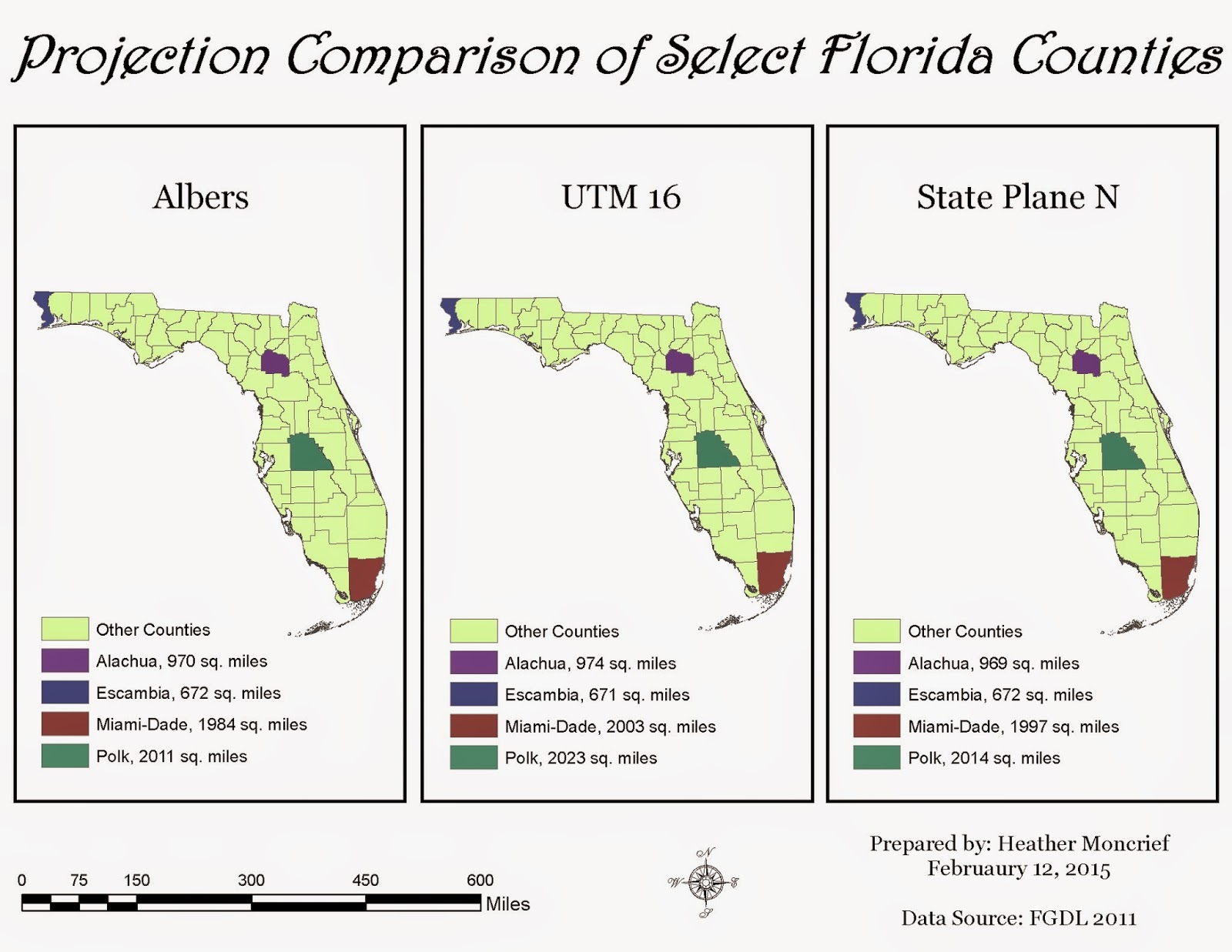Comparison of three projected coordinate systems, Albers, UTM 16, and State Plane N projected onto the state of Florida. Alachua, Escambia, Miami-Dade and Polk Counties are highlighted as examples. Source: FGDL 2011

This week we learned about projections and how they affect the map-making process. I enjoyed making these maps, especially seeing the difference in the projected coordinate systems. This is honestly something I had never considered before. I think it is definitely beneficial that we set up the maps this way, with three on one image, it allows you to be able to see the slight differences in the shape of the state. Showing the area of the counties across all of the maps is very helpful as well, since it shows the slight differences in size among the projections.

I set my maps up very similar to the example provided, because I thought it was set up well and wanted to see if I could teach myself a couple of things while doing the lab. This did add a little bit of time to my lab time since every time you make major changes to your legend, you have to reset the color ramp. I think I set those colors 4 times!

Week 4 - IntroGIS - ArcGIS Online and Map Packages

Information for map package uploaded onto ArcGIS Online for "Use and modify map and tile packages" exercise.

This week's lab exercise was different, because we did not create a map like we have been doing. We also were following instructions straight from ESRI using their Virtual Campus. It was nice that their instructions were easy to follow, similar to our UWF course. The images included in this post show what the packages look like, including the description, properties and access and use constraints. You can edit this information if needed. I really like the fact that sharing the map package is so easy to do, and that you can select who to share it with, which is great for collaborating on projects. It is also nice that you can open up the package directly from the site into ArcGIS for Desktop. 

Information for map package uploaded onto ArcGIS Online for "Optimize a map package" exercise

Week 3 - IntroGIS - Cartography

Topography map of Mexico. Green depicts lower elevations, whereas brown indicated higher elevations. Data Source: UWF, ESRI (2007)

I really enjoyed working on this lab. We made three separate maps: one for the states of Mexico, with a color ramp depicting population sizes; one for showing the major highways, railroads along with primary and major rivers of Central Mexico; and the above topography map. I liked the fact that although we worked with totally different data sets, we mapped relatively the same area. This shows a small sample of the different kinds of information that can be utilized when using a GIS. We used raster data for the first time in order to make the topography map, which was quite interesting to work with. I did realize that I am slightly OCD in the fact that it bothered me greatly that there was no "texture" to the surrounding countries.

Week 2 - IntroGIS - Own Your Map

Map showing the location of the UWF campus within Escambia County, Florida. Source: FGDL2008

I had a lot of fun creating this map. I really like the fact that our instructions allow us to add our own personal touches to the maps that we create. I did have one little time-consuming issue in the beginning with the Overview: Escambia County data frame (inset). I misunderstood the directions and struggled to keep the image within the frame ( I was re-sizing and panning repeatedly). I did finally realize that all I had to do was "Zoom to Layer". I really like that this week's lab built on last week's, reinforcing what we have learned so far. I look forward to improving my skills through the upcoming weeks.

Week 1 - IntroGIS - ArcGIS Overview Lab

Map 1. Population of countries across the globe. Colors coordinate to population size, with teal being least populated and white being most populated. Black squares indicate major cities. Data Source: USGS 2008.

This was my first time working with ArcGIS, and I found it fairly user friendly when following the instructions given. The biggest struggle that I had was with learning how to save the file correctly for later use. I learned the hard way that you cannot rearrange your files after saving and expect for your map to come back up, that you must save again in the new file structure. 

At first I was not happy with the size of the legend for this map, I wanted it larger for better reading, but was not sure how to do so. Luckily, someone posted in our discussion forum how to do so (using the Pan Tool). I also do not like that the first value for the lowest populated countries is -99,999 instead of 0. However, for my first map, I am happy with it overall.